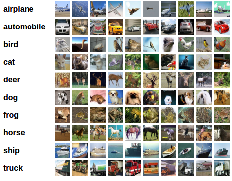
Image classifier - CIFAR10
Goal:
Background:
As part of initial code, following steps are done in order:
- Loading and normalizing the CIFAR10 training and test datasets using torchvision
- Defining a Convolutional Neural Network
- Defining a loss function
- Training the network on the training data
- Testing the network on the test data

In our case, input images are of 32*32 pixels in size, therefore W is 32


Experimental Observations:
Output of average accuracy in different runs : 42% 42 % 42% 42% 41%
2. Using softmax
Code change: return F.log_softmax(x) instead of return x
3. Using variation in input output of convolutional layer
I) input -> conv2d -> relu -> maxpool2d
II) input -> conv2d -> relu -> conv2d -> relu -> conv2d -> relu -> maxpool2d
with small variation in output
Output of average accuracy in different runs: 30% 32% 28% 19%
III) input -> conv2d -> relu -> conv2d -> relu -> conv2d -> relu -> maxpool2d
with large variation in output
Output of average accuracy in different runs: 44% 45% 44% 44%
4. Without pooling
Output of average accuracy in different runs : 56% 52% 54% 54%
5. Using single convolution layer in given code with higher output value
Output of average accuracy in different runs: 58% 57% 57% 56%
I) Using output channel value as 9
Output of average accuracy: 58%
II) Using output channel value as 12
Output of average accuracy: 59%
III) Using output channel value as 24
Output of average accuracy: 60%
IV) Using output channel value as 30
Output of average accuracy: 61%
V) Using output channel value as 40
Output of average accuracy: 63%
6. Using single convolution layer in given code with higher output value and increasing the number of epochs
I) Using number of epochs as 2
Output of average accuracy: 60%
II) Using number of epochs as 4
Output of average accuracy: 66%
III) Using number of epochs as 6
Output of average accuracy: 66%
IV) Using number of epochs as 8
Output of average accuracy: 66%
IV) Using number of epochs as 10
Output of average accuracy: 66%
Challenges faced:


In most of the cases, the value of average percentage varies in different runs. This makes it difficult to precisely differentiate one case with other. However, as the variation was not very large, the approximated values could be used for comparisons.
Analysis:
Based on the observations made,
1. The change in average accuracy with output channel value is seen to be linear as part of point 5 in experiments performed. Increasing the output channel value increased accuracy as follows.

2. The change in average accuracy with number of epochs is seen to be increasing as part of point 6 in experiments performed as follows. It increases initially and then does not bring much change in accuracy.

Code:
Following is the link for final code in GitHub:
Outcome:
On applying the changes to output channel in the code and increasing the epochs, average accuracy of ten classes in CIFAR10 classifier improved from around 56% to 66%
References:
- https://pub.towardsai.net/building-neural-networks-with-python-code-and-math-in-detail-ii-bbe8accbf3d1
- https://www.youtube.com/watch?v=FTr3n7uBIuE&t=2100s
- https://www.youtube.com/watch?v=pDdP0TFzsoQ
Contribution:
- Increasing the output channel after reducing the number of layers increases the performance of the model.
- Looking at the graph drawn as part of analysis we see that increasing the number of epochs can be used to improve the performance of the model. However, after some time it does not bring much change and gives same accuracy on increment. It takes somewhat more time to run the model with this change.


Comments
Post a Comment